What is Bezier simplex fitting?

The Bezier simplex is a high-dimensional generalization of the Bezier curve and Bezier triangle with which we are familiar in computer graphics and computer-aided design. As such 1D and 2D instances of Bezier simplices have a great success in those fields, Bezier simplices of general dimension have excellent flexibility to represent various shapes in arbitrary dimensions. This page introduces the basics of Bezier simplices and their fitting algorithm, along with illustrative applications.

Bezier simplex

Let \(D, M, N\) be nonnegative integers, \(\mathbb N\) the set of nonnegative integers (including zero!), and \(\mathbb R^N\) the \(N\)-dimensional Euclidean space. We define the index set by

\[\mathbb N_D^M = \left\{\mathbf d=(d_1,\ldots,d_M)\in\mathbb N^M\ \Bigg|\ \sum_{m=1}^M d_m=D\right\},\]

and the simplex by

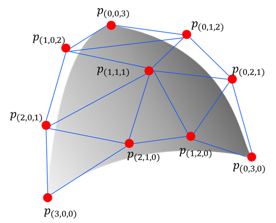
\[\Delta^{M-1} = \left\{\mathbf t=(t_1,\ldots,t_M)\in[0,1]^M\ \Bigg|\ \sum_{m=1}^M t_m=1\right\}.\]

An \((M-1)\)-dimensional Bezier simplex of degree \(D\) in \(\mathbb R^N\) is a polynomial map \(\mathbf b: \Delta^{M-1}\to\mathbb R^N\) defined by

\[\mathbf b(\mathbf t\mid\mathbf p) = \sum_{\mathbf d\in\mathbb N_D^M} \binom{D}{\mathbf d} \mathbf t^{\mathbf d} \mathbf p_{\mathbf d},\]

where \(\mathbf t^{\mathbf d} = t_1^{d_1} t_2^{d_2}\cdots t_M^{d_M}\), \(\binom{D}{\mathbf d}=D! / (d_1!d_2!\cdots d_M!)\), and \(\mathbf p_{\mathbf d}\in\mathbb R^N\ (\mathbf d\in\mathbb N_D^M)\) are parameters called the control points.

Fitting a Bezier simplex to a dataset

Assume we have a finite dataset \(B\subset\Delta^{M-1}\times\mathbb R^N\) and want to fit a Bezier simplex to the dataset. What we are trying can be formulated as a problem of finding the best vector of control points \(\mathbf p=(\mathbf p_{\mathbf d})_{\mathbf d\in\mathbb N_D^M}\) that minimizes the least square error between the Bezier simplex and the dataset:

\[\arg\min_{\mathbf p} \sum_{(\mathbf t,\mathbf x)\in B}\|\mathbf b(\mathbf t\mid\mathbf p)-\mathbf x\|^2.\]

PyTorch-BSF provides an algorithm for solving this optimization problem with the L-BFGS algorithm.

Why does Bezier simplex fitting matter?

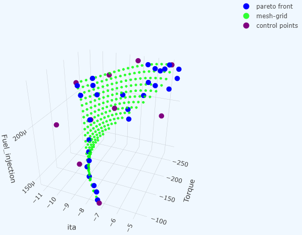
The Bezier simplex can approximate the solution set of “good” multiobjective optimization problems. More precisely, for the weighted sum scalarization problem of any multiobjective strongly convex problem, the map from a simplex of weight vectors to the solution set of weighted sum problems can be approximated by a Bezier simplex. If we find few solutions to such a problem, the entire solution set can be approximated by Bezier simplex fitting. An important application is hyperparameter search of the elastic net.

Approximation theorem

Any continuous map from a simplex to a Euclidean space can be approximated by a Bezier simplex. More precisely, the following theorem holds. See [1] for technical details.

Weakly simplicial problems

Such a map \(\Phi\) arises in, e.g., multiobjective optimization. There exists a continuous map from a simplex to the Pareto set and Pareto front such that the map sends a subsimplex to the Pareto set/front of a subproblem. See [3].

Application 1: Elastic net

Hyper-parameter search. See [3] for technical details.

Strongly convex problems

All unconstrained strongly convex problems are weakly simplicial [3].

Weighted-sum scalarization and solution map

The weighted-sum scalarization \(x^*: \Delta^{M-1}\to\mathbb R^N\) defined by

\[x^*(w)=\arg\min_x \sum_{m=1}^M w_m f_m(x).\]

We define the solution map \((x^*,f\circ x^*):\Delta^{M-1}\to G^*(f)\) by

\[(x^*,f\circ x^*)(w)=(x^*(w),f(x^*(x))).\]

The solution map is continuous and surjective. See [3] for technical details.

Application 2: Deep neural networks

The loss function for the generator is

\[ \begin{align}\begin{aligned}L_D^\mathrm{bCR}&=L_D+\lambda_\mathrm{real}L_\mathrm{real}+\lambda_\mathrm{fake}L_\mathrm{fake},\\L_D&=D(G(z))-D(x),\\L_\mathrm{real}&=\|D(x)-D(T(x))\|^2,\\L_\mathrm{fake}&=\|D(G(z))-D(T(G(z)))\|^2,\\L_D^\mathrm{zCR}&=L_D+\lambda_\mathrm{dis}L_\mathrm{dis},\\L_G^\mathrm{zCR}&=L_G+\lambda_\mathrm{gen}L_\mathrm{gen},\\L_G&=-D(G(z)),\\L_\mathrm{dis}&=\|D(G(z))-D(G(T(z)))\|^2,\\L_\mathrm{gen}&=\|G(z)-G(T(z))\|^2.\end{aligned}\end{align} \]

Statistical test for weakly simpliciality

When problem class is unknown. See [4] for technical details.

References

Kobayashi, K., Hamada, N., Sannai, A., Tanaka, A., Bannai, K., & Sugiyama, M. (2019). Bézier Simplex Fitting: Describing Pareto Fronts of Simplicial Problems with Small Samples in Multi-Objective Optimization. Proceedings of the AAAI Conference on Artificial Intelligence, 33(01), 2304-2313. https://doi.org/10.1609/aaai.v33i01.33012304
Tanaka, A., Sannai, A., Kobayashi, K., & Hamada, N. (2020). Asymptotic Risk of Bézier Simplex Fitting. Proceedings of the AAAI Conference on Artificial Intelligence, 34(03), 2416-2424. https://doi.org/10.1609/aaai.v34i03.5622
Mizota, Y., Hamada, N., & Ichiki, S. (2021). All unconstrained strongly convex problems are weakly simplicial. arXiv:2106.12704 [math.OC]. https://arxiv.org/abs/2106.12704
Hamada, N. & Goto, K. (2018). Data-Driven Analysis of Pareto Set Topology. Proceedings of the Genetic and Evolutionary Computation Conference, 657-664. https://doi.org/10.1145/3205455.3205613